Understanding the Standard Normal Distribution and Z-Scores

Expert reviewed • 21 July 2024 • 16 minute read

calculate probabilities and quantiles associated with a given normal distribution using technology and otherwise, and use these to solve practical problems
- visually represent probabilities by shading areas under the normal curve, eg identifying the value above which the top 10% of data lies
use collected data to illustrate the empirical rules for normally distributed random variables
- apply the empirical rule to a variety of problems

Note:

Video coming soon!

What is the Standard Normal Distribution?

The standard normal distribution is a special case of the normal distribution where the mean $(\mu)$ is $0$ and the standard deviation $(\sigma)$ is 1. It is a continuous probability distribution that is symmetric about the mean.

The PDF of the Standard Normal Distribution

As discussed in the previous module, the PDF of a continuous probability distribution describes the likelihood of a continuous random variable taking on a particular value. To determine the PDF of a standard normal distribution, we must first let $z$ be the standard normal variable. We do this so that calculating z-scores becomes easier (calculating z-scores will be explored in the next chapter). As such, the formula to determine the PDF of the standard normal distribution is given by:

\phi(z) = \frac{e^{-\frac{z^2}{2}} }{\sqrt{2\pi}}

where,

$z$ represents a value you are calculating the probability density for.
$\frac{1}{\sqrt{2\pi}}$ is a normalisation constant, which ensures that the total area under the curve of the PDF equals $1$ . This is important because the total probability outcome must equal $1$ .
$-\frac{z^2}{2}$ in the exponent makes the function a bell-shaped curve that is symmetric around zero.

This formula must be understood to grasp a solid concept of normal distributions. However, during HSC exams, you are rarely required to use it, as questions will generally ask you to use a given z-score table to help you solve the given problem. Z-scores tables will be explained later in this chapter.

Graphing the PDF of the Standard Normal Distribution

The graph of the PDF of a standard normal distribution has a specific and unique bell-curve shape. Modelled on the PDF’s equation stated above, we see the graph look something like the following:

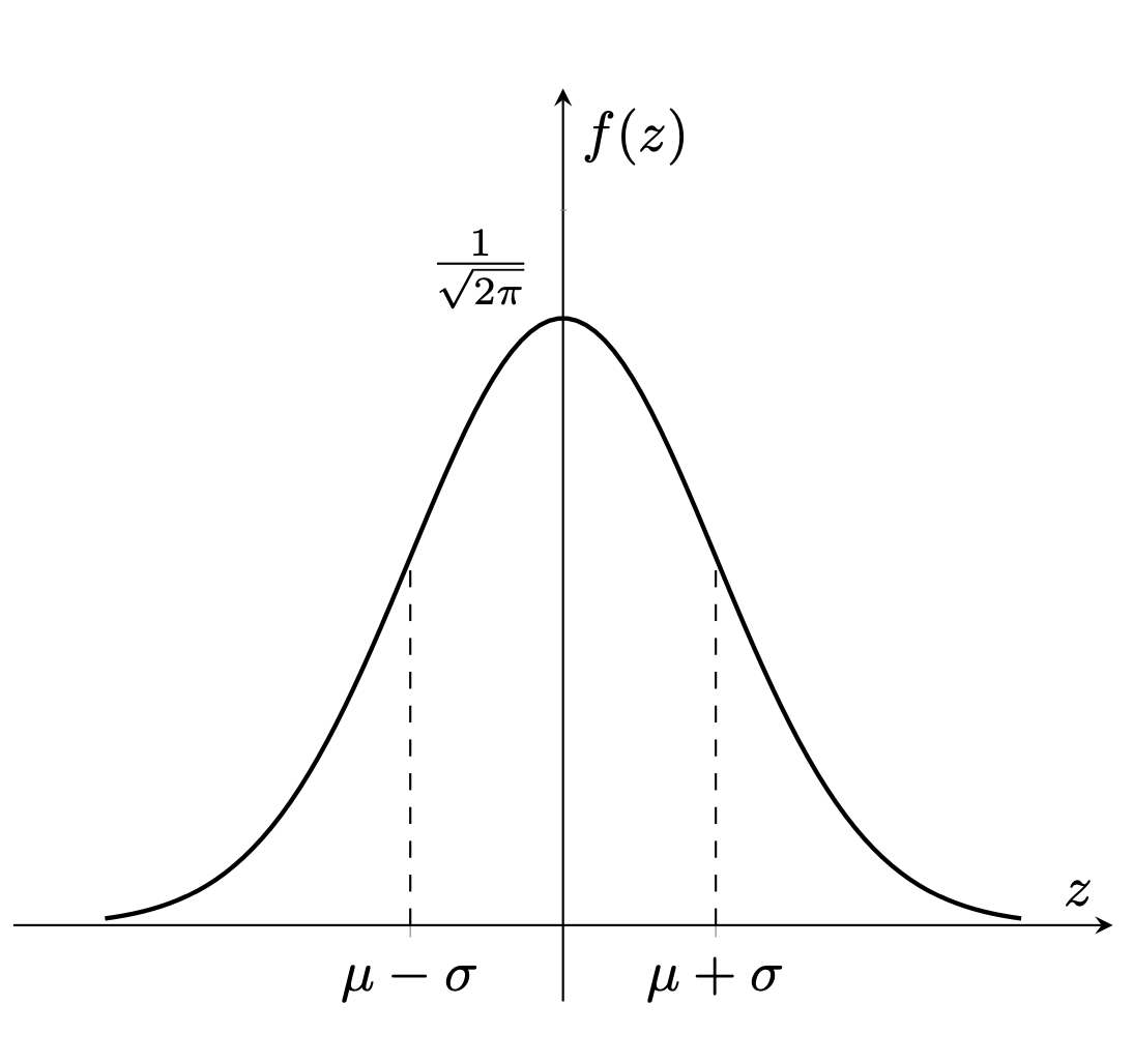
The bell shape of the standard normal distribution curve means that values close to the mean (which in this case is zero) are more probable than values far from the mean.

Important Features of the Graph

Mean $(\mu)=0$
- This is the centre of the distribution and the peak of the bell curve.
Standard Deviation $(\sigma)=1$
- This measures the spread or dispersion of the distribution.
- Points on the curve are spread one standard deviation away from the mean.
The curve is symmetric about the $y$ -axis
The $y$ -intercept $= \frac{1}{\sqrt{2\pi}}$

The Cumulative Distribution Function of The Standard Normal Distribution

The CDF of the standard normal distribution represents the probability that a standard normal random variable $Z$ is less than or equal to a particular value $x$ . The value of the CDF of the standard normal distribution is given by:

\Phi(x) = \frac{1}{\sqrt{2\pi}} \int_{-\infty}^x e^{-\frac{1}{2}z^2} \, dt

Where,

$\Phi(x)$ represents the cumulative distribution function of the standard normal distribution at the value $x$ .
The integral calculates the area under the curve of the standard normal distribution from $-\infty$ to $x$ .

It is important to note that the limits given in the equation above are $-\infty$ and $x$ . However, the expression can be manipulated to range between the limits $x$ to $\infty$ , or $x$ to an alternate value contained in the normal distribution. However, when we come to calculate the CDF or the probability of the function, we can use a z-score table.

Calculating Probabilities Using Z-Scores

A z-score is a measure that describes the position of a data point in terms of standard deviations from the mean. In the context of the standard normal distribution, a z-score of $x$ refers to the value $x$ standard deviations away from the mean. This means that instead of using the formula above to calculate the probability of a score $x$ when in the form $P(Z\leq x)$ , we can use the z-score table below.

Z-Score Table:

Z-Score Table

We can use this table, by looking at the corresponding z-score for a given value of $x$ . For example, if we are given a score of $2.0$ for the expression $P(Z\leq2)$ and we are asked to find the corresponding z-score. From the table, using the left-hand column we can see that a value of $2.0$ is $0.9772$ . This means that the probability of finding a score, between $-\infty$ and 2 standard deviations away from the mean, is $97.72\%$ .

The bell-curve-graph of the given example above is as follows:

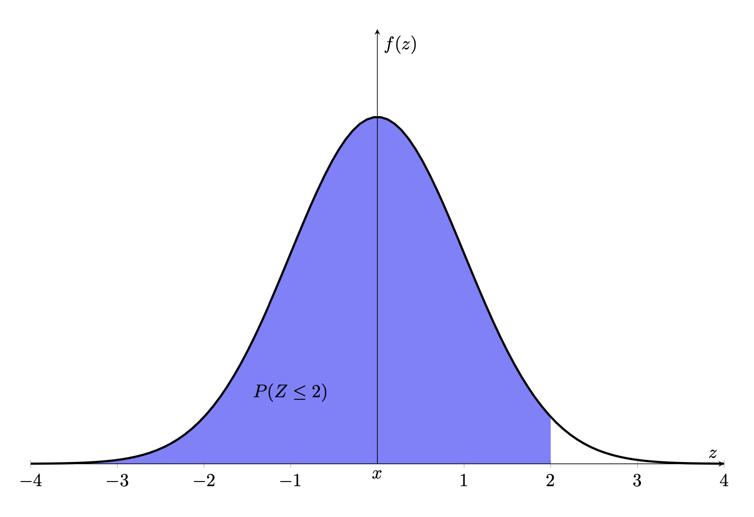
We can see from the graph that the area between $-\infty$ and $2$ is shaded. This represents the cumulative probability up to $x=2$ , indicating the probability of finding a score less than the random variable $Z$ .

It is important to know that when the inequality sign is reversed, we must calculate the probability by finding the z-score in the form $P(Z\leq x)$ , and then subtracting the found value from 1. We do this because the entire area under the curve is 1.

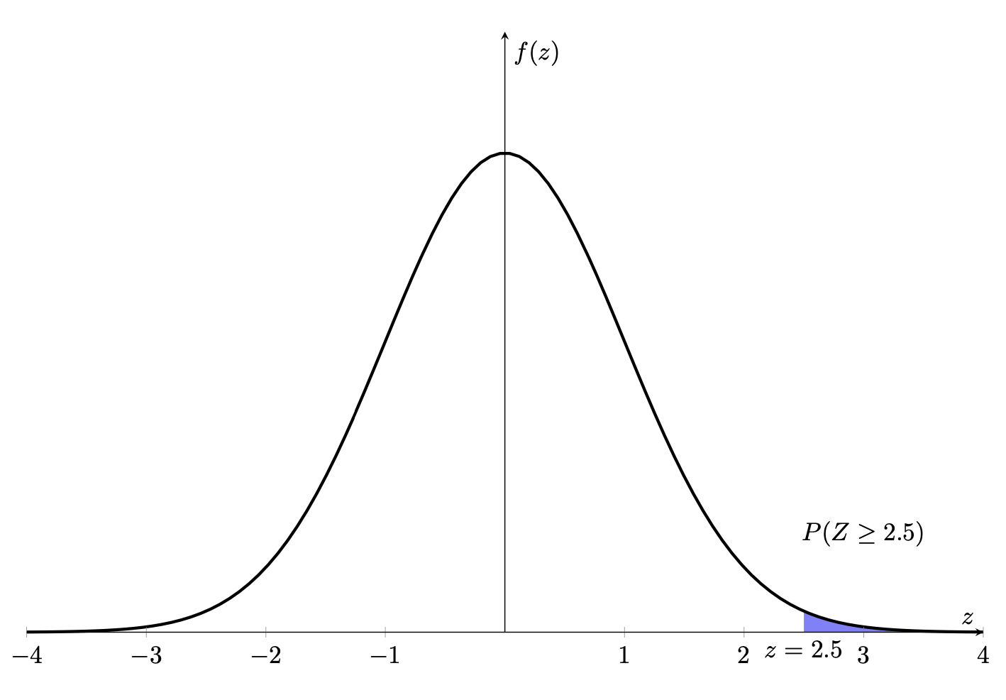
Practice Question 1

Using the following z-score table, determine $P(Z\geq 2.5 )$ , and graph the corresponding bell curve. When you create the graph, ensure you shade the identified area.

Z-Score Table:

z	.0	.1	.2	.3	.4	.5	.6	.7	.8	.9
0.	0.5000	0.5398	0.5793	0.6179	0.6554	0.6915	0.7257	0.7580	0.7881	0.8159
1.	0.8413	0.8643	0.8849	0.9032	0.9192	0.9332	0.9452	0.9554	0.9641	0.9713
2.	0.9772	0.9821	0.9861	0.9893	0.9918	0.9938	0.9953	0.9965	0.9974	0.9981
3.	0.9987	0.9990	0.9993	0.9995	0.9997	0.9998	0.9998	0.9999	0.9999	1.0000

To determine the probability $P(Z\geq 2.5)$ we must first reverse the inequality sign and find the given value using the z-score table above. Using the table, we can see that the corresponding probability of a z-score of $2.5$ is $0.9938$ , or $99.38\%$ .

As stated in the module, $P(Z\leq 2.5)=1-P(Z\geq2.5)$ . Thus we can determine the probability being asked for.

P(Z\leq 2.5)=1-0.9938\\=0.0062

$\therefore$ The probability of $P(Z\leq 2.5)$ is $0.0062$ or $0.62\%$

Now, to graph this, we must take the standard normal distribution bell curve, and shade the area from $x=2.5$ onwards.

What is the Empirical Rule?

The Empirical Rule, also known as the 68-95-99.7 rule, describes the proportion of scores that are distributed in a normal distribution. It states that:

$68\%$ of the data falls within one standard deviation of the mean

\mu\pm1\sigma

$95\%$ of the data falls within two standard deviations of the mean

\mu\pm2\sigma

$99.7\%$ of the data falls within three standard deviations of the mean

\mu\pm3\sigma

This rule is used when we are asked to determine the probability of a score of $1,2$ or $3$ standard deviations within the mean. This way a z-score table is not needed to determine the answer. It is important to note that the empirical rule is just a general guideline that provides a rough estimate of the spread of data around the mean of a normal distribution. It is not precise enough to use in some scenarios, hence why we use z-score tables, which are far more accurate.

Mean and Variance of the Normal Distribution

Up Next

General Normal Distributions & Z-Scores

Return to Module 10: Continuous Probability Distributions