Understanding General Normal Distributions and Standardisation
Expert reviewed • 04 March 2025 • 9 minute read
- understand and calculate the 𝑧-score (standardised score) corresponding to a particular value in a dataset
- use the formula 𝑧 =𝑥−𝜇𝜎 , where 𝜇 is the mean and 𝜎 is the standard deviation
- describe the 𝑧-score as the number of standard deviations a value lies above or below the mean
- use 𝑧-scores to compare scores from different datasets, for example comparing students' subject examination scores
- use collected data to illustrate the empirical rules for normally distributed random variables
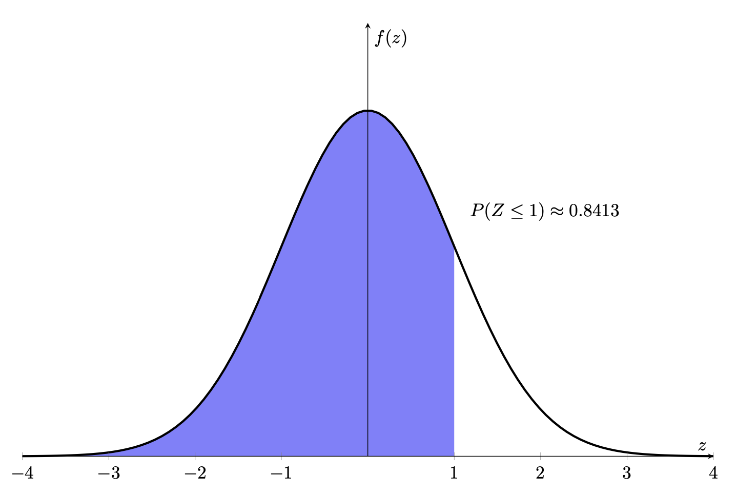
- sketch the graphs of and the probability density function for the normal distribution using technology
- use 𝑧-scores to make judgements related to outcomes of a given event or sets of data
Note:
Video coming soon!
What is the General Normal Distribution?
The general normal distribution is a continuous probability distribution that is symmetrical around its mean. In the previous chapter, we discussed a type of normal distribution known as the standard normal distribution. The standard normal distribution is a special case of the normal distribution with a mean of and a standard deviation of . This chapter focuses on normal distributions that are symmetrical around values other than .
Problems involving normal distributions are solved by using the same methods outlined in the previous chapter - using z-score tables. However, when dealing with general normal distributions, we must find the z-score from a given mean and standard deviation. This is done through a method called standardisation.
What is Standardisation?
Note:
Video coming soon!
Standardisation involves converting a normal distribution with a mean and standard deviation into a standard normal distribution (with mean and standard deviation ). This is done, so we can apply the process of using z-score tables to determine a measure of probability. The process of standardisation is defined by the z-score formula, which is given by:
This formula standardises z-score values, so they can be measured according to the same scale, being the standard normal distribution, with a mean of and a standard deviation of . As we know from the previous chapter, a sore indicates how many standard deviations a data point is from the mean. It is important to note that:
- Positive z-scores refer to values above the mean
- Negative z-score values refer to values below the mean
Solving Problems Using Standardisation
As discussed in the previous chapter, to determine the probability of certain values or ranges of a standard normal distribution, we must find corresponding values using a z-score table and graph the given bell curve. However, when dealing with a general normal distribution (a normal distribution with a mean value other than ), we must apply the process of standardisation, as seen above, before calculating the probability.
Practice Question 1
A class of students sit a math test graded out of marks. A student wishes to asses his performance against that of the rest of his class. The mean of all the test results was and the standard deviation of the results was . This student achieved a score of . Determine the student's performance on the test, relative to the average performance of all students who took the test. Additionally, create a relevant graph to support your answer. Use the following z-score table to assist you with any calculations.
| z | .0 | .1 | .2 | .3 | .4 | .5 | .6 | .7 | .8 | .9 |
|---|---|---|---|---|---|---|---|---|---|---|
| 0. | 0.5000 | 0.5398 | 0.5793 | 0.6179 | 0.6554 | 0.6915 | 0.7257 | 0.7580 | 0.7881 | 0.8159 |
| 1. | 0.8413 | 0.8643 | 0.8849 | 0.9032 | 0.9192 | 0.9332 | 0.9452 | 0.9554 | 0.9641 | 0.9713 |
| 2. | 0.9772 | 0.9821 | 0.9861 | 0.9893 | 0.9918 | 0.9938 | 0.9953 | 0.9965 | 0.9974 | 0.9981 |
| 3. | 0.9987 | 0.9990 | 0.9993 | 0.9995 | 0.9997 | 0.9998 | 0.9998 | 0.9999 | 0.9999 | 1.0000 |
Solution
The first step to solving this problem is to apply the process of standardisation. From the question we know that and .
Now that we have standardised the data given, we can see that the z-score of this distribution is . Thus, we can use the z-score table provided in the question to determine the probability. From the table we can see that:
This means that the student scored better than approximately of students in the class on the exam. We can graph this by shading the area under a bell-curve graph, between and .